Model and methods

These pages state the equations SIMPLE solves, as the code solves them, with the implementing routine for each.

• Guiding-centre model
  • Phase-space Lagrangian
  • Canonical form
  • Normalisation
  • Invariants and trapping parameter
  • References
• Coordinates and field representation
  • Reference and integration coordinates
  • Canonical flux coordinates (integ_coords = 0)
  • Boozer coordinates (integ_coords = 2)
  • Meiss coordinates (integ_coords = 3)
  • Albert coordinates (integ_coords = 4)
  • Field sources
  • References
• Integrators
  • Step size
  • Symplectic schemes
  • Adaptive Runge–Kutta (integmode = 0)
  • Loss crossing inside a step
  • Failure recovery
  • References
• Collisions
  • Scope and splitting
  • Coefficients
  • Discrete step
  • Monoenergetic Lorentz mode
  • Random streams
  • References
• Orbit classification
  • Footprints
  • Class codes
  • \(J_\parallel\) and topological classifiers
  • Fractal classifier
  • References
• Wall intersection
  • Loss boundaries
  • Segment–triangle test
  • Query gate
  • Accuracy
  • References
• Heat-load estimators
  • Marker power and energy
  • Flux on flux-surface bins
  • Load on STL triangles
  • Accuracy
  • References
• Full orbit, SPECTRE and GPU objective
  • Full-orbit tracing
  • SPECTRE equilibria
  • GPU loss objective
  • References

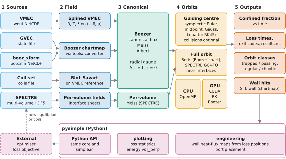
Phases of a simple.x run.

Phases of a run

1. Field. Read a VMEC equilibrium, a chartmap, a coil file or a SPECTRE equilibrium; construct coordinates in which the guiding-centre Lagrangian is canonical and spline \(A_\vartheta, A_\varphi, h_\vartheta, h_\varphi, B\) (Coordinates and field representation).

2. Sampling. Draw start positions in reference coordinates with speed \(v_0\) and pitch \(\lambda\) (Running SIMPLE).

3. Tracing. Advance each marker in its own OpenMP iteration with the selected integrator (Integrators), optionally followed by a Monte Carlo collision step per microstep (Collisions), until it crosses the loss boundary or the wall (Wall intersection) or reaches trace_time.

4. Classification (optional): label regular and chaotic orbits from their Poincaré footprints (Orbit classification).

5. Output (Outputs).

Assumptions

• Test particles in a static magnetic field; no electric field.

• Guiding-centre motion to first order in \(\rho_L/L\); the guiding centre, not the particle, defines losses and wall hits. Full-orbit tracing is an alternative model (Full orbit, SPECTRE and GPU objective).

• Non-relativistic (rmu = 1e8 in src/params.f90).

• Collisions are a test-particle operator with a Maxwellian background of electrons and two ion species, using alpha-particle mass and charge (Collisions).

• A marker is lost when it leaves the last closed flux surface or the chartmap domain, or hits an STL wall.